If you got here via a link to the slides
Please check out the full git repository for the presentation notebook as well as other example notebooks.
https://github.com/OttoStruve/ipython_notebook_presentation/tree/gsps
This presentation is actually adapted from one given by Joshua Barratt at LinuxCon
from IPython.display import YouTubeVideo
YouTubeVideo('XkXXpaVpNSc', width=853, height=480)
Open Source FTW!
Outline
- What is the notebook
- OMG it's the best
- Quick Demo
- IPython Ecosystem (2.0 Caveat)
- Why is it awesome
- Literate Code
- Sharing
- Rapid Prototyping/Exploring/Learning
Terminal(Editor <-> Renderer) -> Emailvs Cyclic
- Blogging
- Workflows (edit, share, publish)
- Under the hood
ipynb - HTML
- Gist + nbviewer
- Under the hood
- Demos
- Code Mentorship (sets, objects, katas)
- Runbooks
- Log analysis epic
- Shell scripting demo
- Churn analysis
- Latency Heatmap
- Extending
- It came from inside the presentation!
What is the notebook?
A "browser-based interactive computing environment"
Why are we talking about it today?
- Extremely useful tool, like IT WILL CHANGE YOUR LIFE useful.
- Makes the (powerful) python data/science/module ecosystem even more powerful
- If you code, (even not in python), sysadmin, write documentation, blog, do any analysis or visualization, you might get a lot out of the notebook.
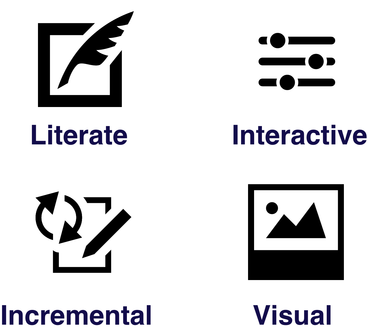
Why It's Great
These attributes will come up over and over as we explore this tool.
"Literate Computing"
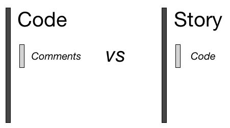
This is a big part of where the title comes from: it's about the story more than the software.
IPython's founder, Fernando Perez @fperez_org has a blog post on this concept.
Here's and example
Enough Meta: Let's Install It:
Install Anaconda
- Everything* you need gets installed
- Easy to install additional packages using the
condautility Even more packages available through Binstar
*Well, almost everything
If you're morally opposed to Continuum Analytics
you can use pip install too.
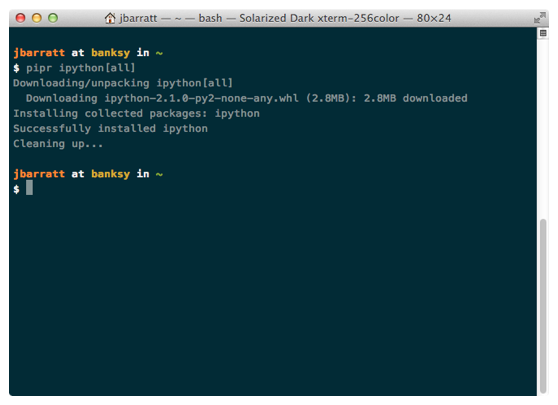
pip install ipython[all] Simple as that.*
*Dependencies can be painful, YMMV.
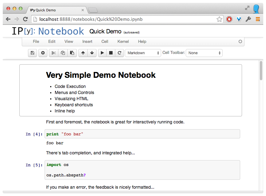
Run 'ipython notebook'
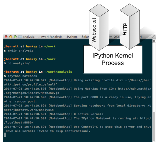
Browser Launches
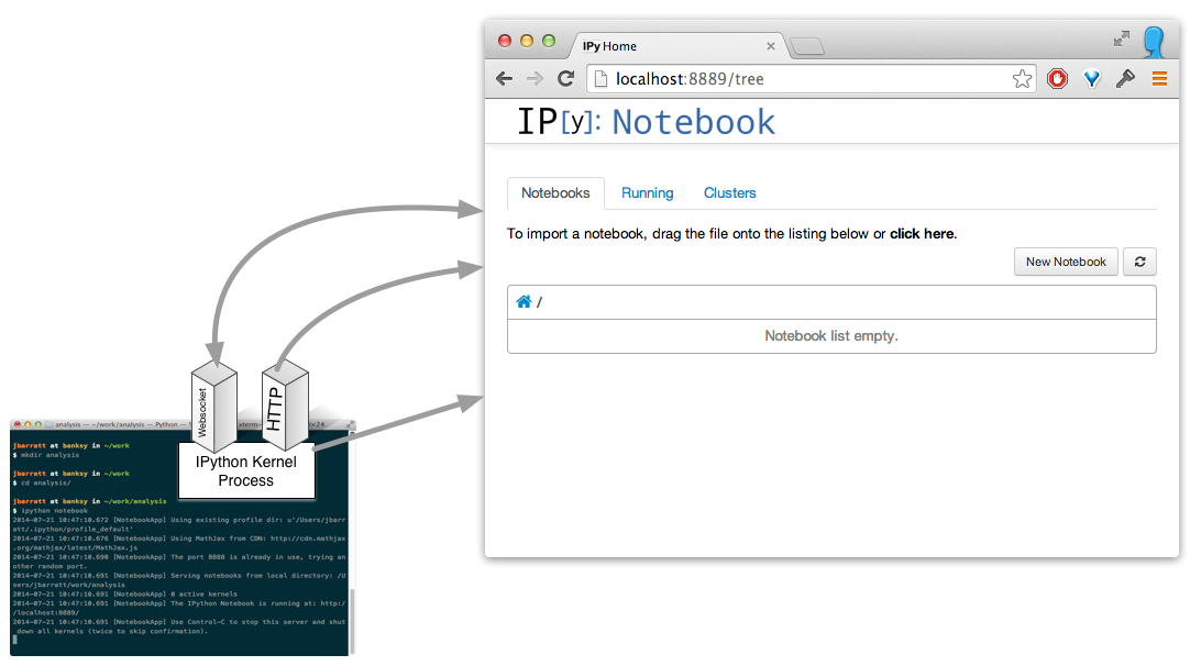
Build a notebook
(Actually, it's a process per open notebook.)
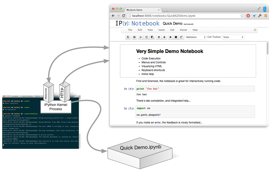
Run A Cell
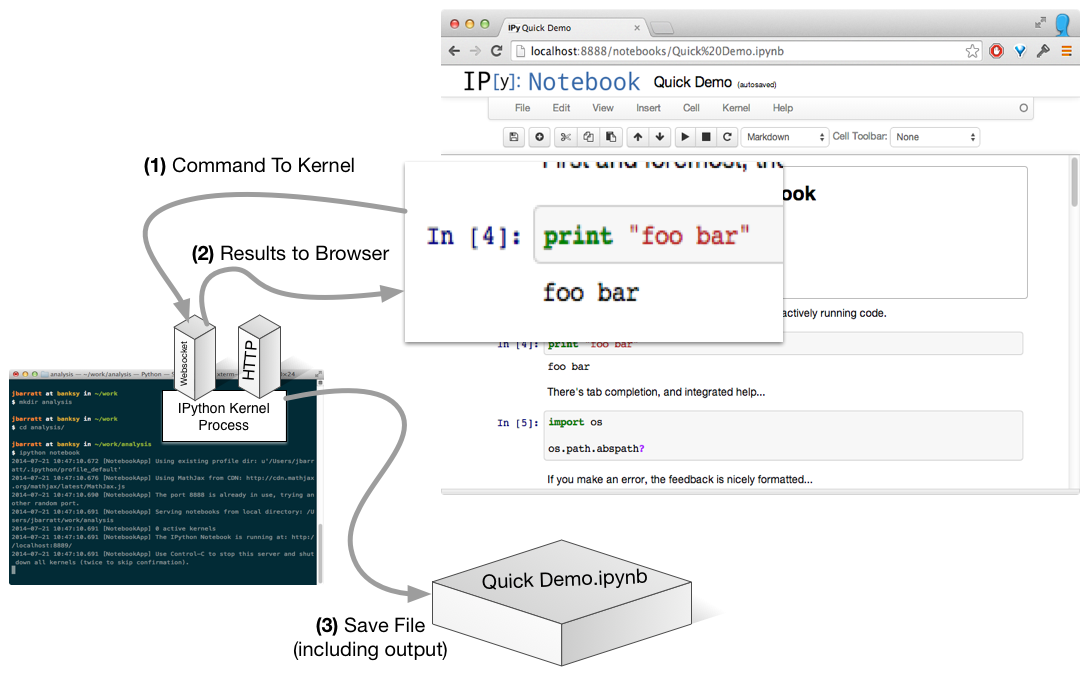
No Need To Be Local...
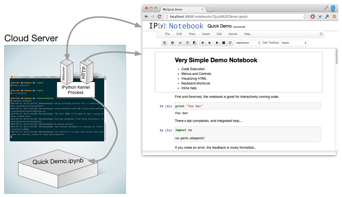
Demo Time

Notebook Workflows: The Big Picture
Not covered today but cool; clustering capabilities
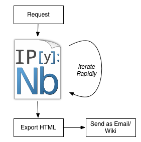
How I Fell: Report Workflow v1
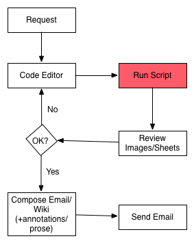
Problems:
- slow (read whole data file each time, lots of context switching)
- version controlled analysis, but not commentary, difficult to 'go back to'
- Automating requires non-trivial additional dev
Report Workflow now()
Speedups primarily from no context switching, interactivity, and reusable data loading.
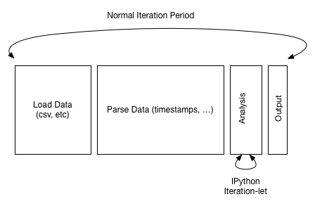
Reproducible, literate, annotatable, auditable.
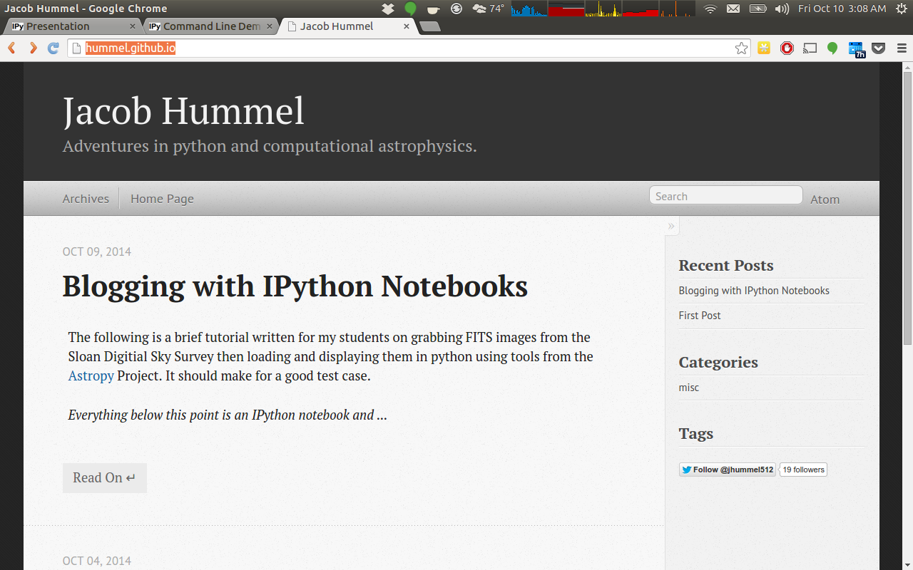
An Example of Iterative Workflow
Viewing and manipulating FITS images in Python
We'll need to import some basic modules to do this; note that %matplotlib inline causes images to appear in the notebook.
import numpy as np
import matplotlib as mpl
import matplotlib.pyplot as plt
%matplotlib inline
In order to handle FITS images in python, we'll need the fits module from astropy:
from astropy.io import fits
The following is optional, and will only work if you have Seaborn installed on your machine, but is a significant improvement over the matplotlib defaults.
- Linux:
conda install -c mutirri seaborn - OSX:
conda install -c asmeurer seaborn
import seaborn as sns
sns.set_context('poster')
sns.set_style('white')
Downloading the data
Go to the SDSS website and download the image of your choice from the SDSS catalog. Here we'll use M42, the Orion Nebula, which looks like this:
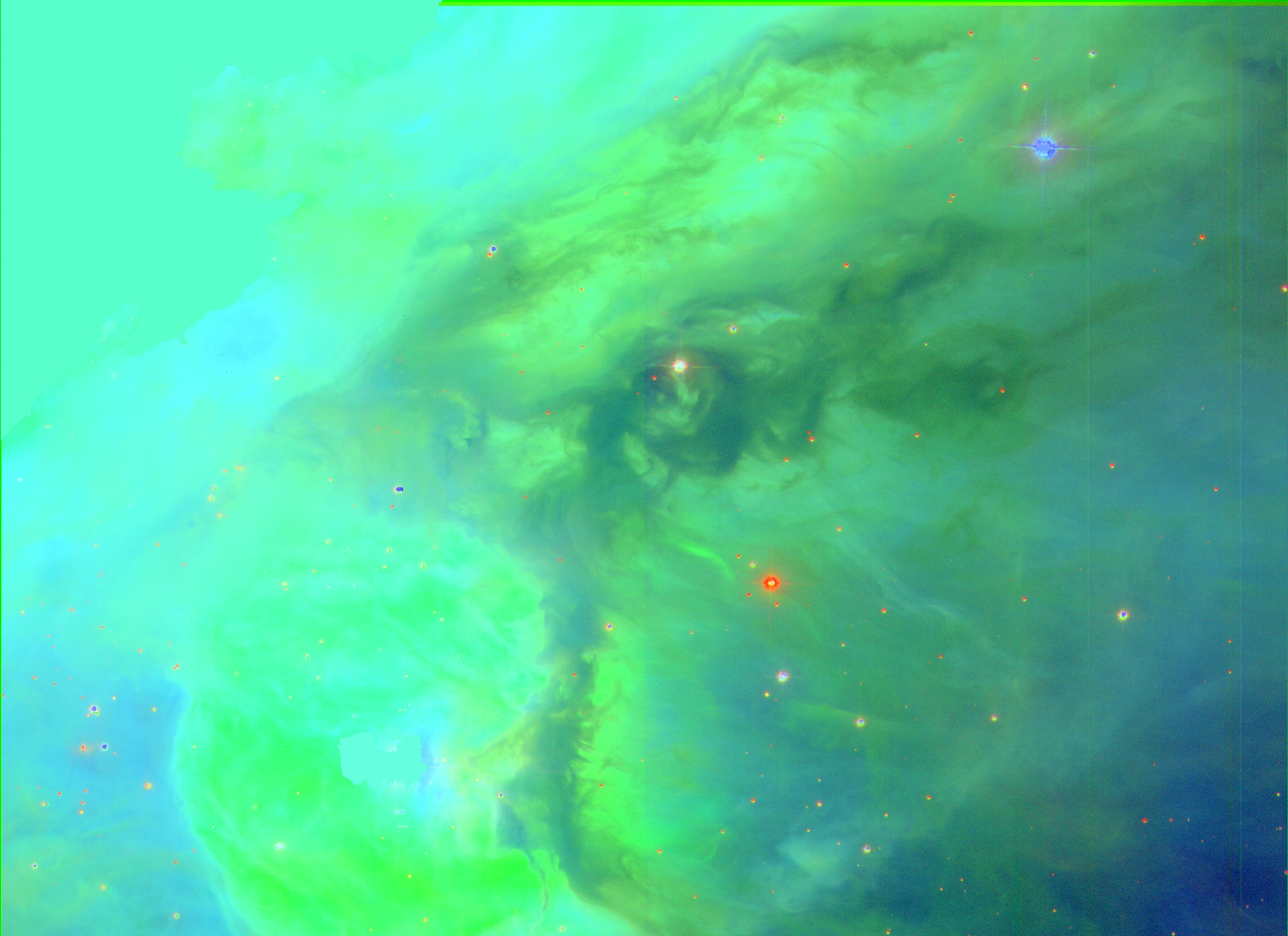
You will need to unzip the files!!! The FITS images you download will be compressed (with a .gz or .bz2 extension). You'll need to extract the file using the program of your choice before proceeding.
Opening FITS files and loading the image data
Let's open the g-band FITS file and find out what it contains.
hdu_list = fits.open("data/frame-g-006073-4-0063.fits")
hdu_list.info()
Generally the image information is located in the PRIMARY block. The blocks are numbered and can be accessed by indexing hdu_list.
image_data = hdu_list[0].data
You data is now stored as a 2-D numpy array. Want to know the dimensions of the image? Just look at the shape of the array.
print(type(image_data))
print(image_data.shape)
At this point, we can just close the FITS file. We have stored everything we wanted to a variable.
hdu_list.close()
SHORTCUT
If you don't need to examine the FITS header, you can call fits.getdata to bypass the previous steps.
image_data = fits.getdata("data/frame-g-006073-4-0063.fits")
print(type(image_data))
print(image_data.shape)
Let's get some basic statistics about our image
print('Min:', np.min(image_data))
print('Max:', np.max(image_data))
print('Mean:', np.mean(image_data))
print('Stdev:', np.std(image_data))
Viewing the image
plt.imshow(image_data, cmap='afmhot', origin='lower')
plt.colorbar()
# To see more color maps go to http://wiki.scipy.org/Cookbook/Matplotlib/Show_colormaps

Unforturnately, we can't really see much here because of the color range. Lets adjust that manually and see what happens.
Plotting a histogram
To make a histogram with matplotlib.pyplot.hist(), you need to cast the data from a 2-D to array to something one dimensional.
Here we'll use the iterable python object image_data.flat.
print(type(image_data.flat))
NBINS = 1000
with sns.axes_style("darkgrid"):
    histogram = plt.hist(image_data.flat, NBINS)

plt.imshow(image_data, cmap='afmhot', origin='lower')
plt.clim(0,30)

Displaying the image with a logarithmic scale
NBINS = 1000
with sns.axes_style("darkgrid"):
    histogram = plt.hist(image_data.flat, NBINS)
    plt.yscale('log', nonposy='clip') #Same histogram, just with logarithmic scaling on the y-axis.

To get a logarithmically scaled image, we need to load the LogNorm object from matplotlib.
from matplotlib.colors import LogNorm
plt.imshow(image_data, cmap='afmhot', norm=LogNorm(), origin='lower')

Why was that cool?
- Interactive & Exploratory.
- Scroll back up, re-review JSON, go another route
- Cached all the things
- Not hitting twitter a bunch (rate limits, etc)
- Static data set (not changing every time you run the code)
- Can even keep developing while on conference wifi (oohhhhhh)
- Easy to keep around as a log for future experiments
- Easy to take that learning and 'bake' it into something more permanent
The "IPython" in "IPython Notebook"`: Interactive Python
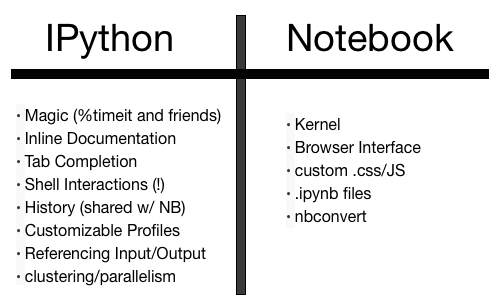
The Future
Skills port to the IPython console
[jhummel@r900-4 ~]$ ipython
Python 2.7.8 |Anaconda 2.0.1 (64-bit)| (default, Aug 21 2014, 18:22:21)
Type "copyright", "credits" or "license" for more information.

IPython 2.2.0 -- An enhanced Interactive Python.
Anaconda is brought to you by Continuum Analytics.
Please check out: http://continuum.io/thanks and https://binstar.org
?         -> Introduction and overview of IPython's features.
%quickref -> Quick reference.
help      -> Python's own help system.
object?   -> Details about 'object', use 'object??' for extra details.

In [1]: import pyGadget as pyg

In [2]: pyg.
pyg.analyze      pyg.hdf5         pyg.sim          pyg.units
pyg.constants    pyg.multiplot    pyg.sink         pyg.visualize
pyg.coordinates  pyg.nbody        pyg.snapshot
pyg.halo         pyg.plotting     pyg.sph
Interactive Gotcha: Single Namespace
As you recall:
So what happens when you do...
x = 5
x
# I ran this cell a few times
x += 1
x
IPython Magic: Development Powertools
Which method is faster?
# make a big array of random numbers
x = np.random.random(500)
# Plan A: iterate through and add them up
def addr(numbers):
    tot = 0.
    for entry in numbers:
        tot += entry

# Plan B: use numpy.sum()

# %timeit is IPython Magic to do a quick benchmark
%timeit addr(x)
%timeit np.sum(x)
%lsmagic
Don't Panic
%%writefile?

    %writefile [-a] filename
    Write the contents of the cell to a file.
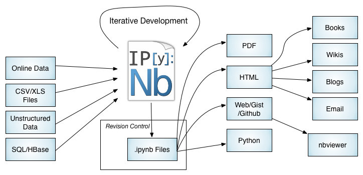
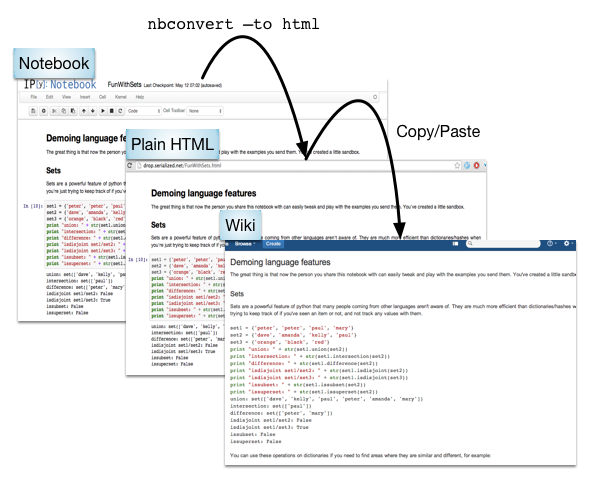
Exporting
ipynb format is clean, readable JSON, which inlines any output results, including base64'd images.
...
{
 "cell_type": "markdown",
 "metadata": {
  "slideshow": {
   "slide_type": "slide"
  }
 },
 "source": [
  "# Magic can be magical"
 ]
},
...
Great Notebook Use Cases
There are many use cases where the notebook makes a lot of sense to use. Here are a few illustrated examples:
- Code Mentorship
- Documentation/Runbooks
- Data Normalization (+ Inline Error Resolution)
- Data Analysis, Portland Example
- Blogging
- Wiki'ing...
We won't go into them all for time, but a few highlights:
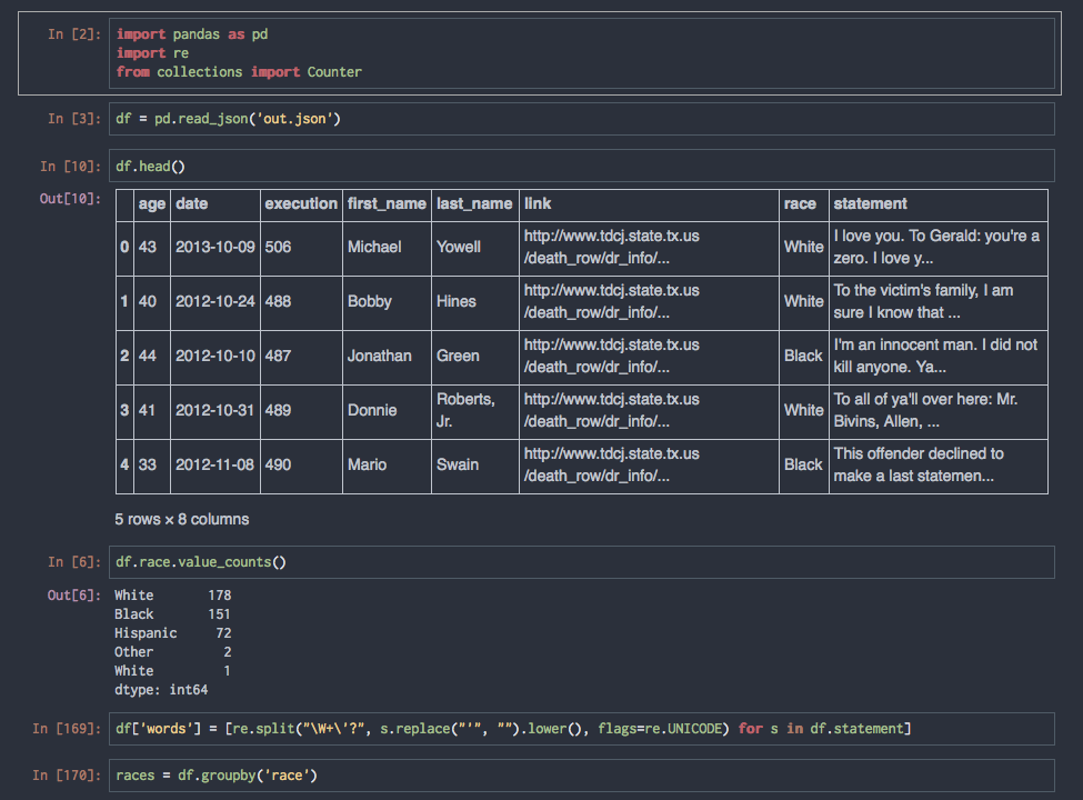
Use Case: Data Analysis
This is the gateway drug that gets many people into IPython Notebook. It's the real sweet spot between what makes Python great (pandas, scikit*, numpy, matplotlib, etc) and IPython Notebook great (Literate, Visual, Interactive, Iterative.)

Did I permanenently ruin your ability to hear the term 'big data' without thinking of this? You're welcome.
Use Case: Code Mentorship

Because you can't always pair...
Use Case: Document ALL THE THINGS

Use Case: Wiki Publishing
Also can work for HTML emails, etc.
Rich Objects
You can also define additional __repr__()-type methods on custom objects.
This has all kinds of fun possibilities.
_repr_html_(), svg, png, jpeg, html, javascript, latex.
class FancyText(object):
    def __init__(self, text):
        self.text = text

    def _repr_html_(self):
        """ Use some fancy CSS3 styling when we return this """
        style=("text-shadow: 0 1px 0 #ccc,0 2px 0 #c9c9c9,0 3px 0 #bbb,"
               "0 4px 0 #b9b9b9,0 5px 0 #aaa,0 6px 1px rgba(0,0,0,.1)")

        return '<h1 style="{}">{}</h1>'.format(style, self.text)

FancyText("Hello GSPS!")
IPython (& Notebook) Customization
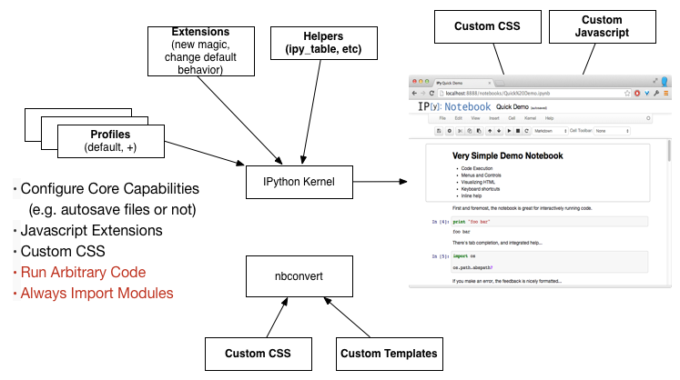
See more on Profiles, Javascript Extensions, IPython Extensions, and nbconvert Templates
Javascript, Huh, What is it good for
Customizing the UI
IPython.toolbar.add_buttons_group([
            {
                id : 'toggle_codecells',
                label : 'Toggle codecell display',
                icon : 'icon-list-alt',
                callback : toggle
            }
      ]);
And more...
Turns out, a lot! You can execute anything you can run in an IPython Notebook cell.
IPython.notebook.kernel.execute("!rm -rf /")
Demo Of a less scary example
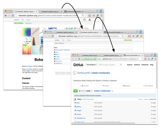
Sharing Notebooks
Oh, one more thing
IT CAME FROM INSIDE THE NOTEBOOK

- Highly technical decks can be created quickly
- Collaboration features are still quite useful
- Check It Out
Building slides
- Turn on the 'slideshow' cell toolbar
- Types:
- Slide: start a new slide
-: Continue a slide- Sub-Slide: Make a 'down' slide
- Fragment: Make a 'bullet' type incoming slide
- Skip: keep in the notebook, not the deck
- Notes: speaker notes
!ipython nbconvert Presentation.ipynb --to slides
Other Resources
Try It Online
Installing
- Anaconda OR
$ pip install ipython[all](brew install python) OR- docker-ipython
- Preloaded with lots of sometimes challenging-to-install packages like Pattern, NLTK, Pandas, NumPy, SciPy, Numba, Biopython...
Learning More
- Slides will be up on the GSPS site later.
- Complete source for this presentation is available on github!
- A Gallery of Interesting IPython Notebooks
- Extensions
- nbviewer (good way to discover organically)
- Pandas/numpy, Statsmodels, Matplotlib, bokeh, vincent, scikit-learn, scikit-image, .... (F150!)
- Talk to me!
Credits
- Quill designed by Simple Icons from the Noun Project,
- Settings designed by Clément thorez from the Noun Project,
- Photo designed by Simple Icons from the Noun Project,
- Recurring Edit designed by Lemon Liu from the Noun Project
- Cover page texture from grungetextures via Flickr.